The boot package in R makes bootstrapping easy – but the format of the output is somewhat of a nightmare. Here, I talk through a small function to extract your boot confidence intervals in a more user-friendly format. If you are new to functions, this could be a good example to get a feel for how they work.
library(boot)
library(tidyverse)
Let’s say we have some sample data of N = 200. We’ve got 4 predictors x1-x4 and an outcome variable y. Predictors x1-x3 and outcome y are continuous, while x4 is binary:
head(data)## # A tibble: 6 × 5
## x1 x2 x3 x4 y
## <dbl> <dbl> <dbl> <dbl> <dbl>
## 1 2.33 2.21 1.25 1 6.6
## 2 5 1.05 1 2 6.2
## 3 4 1.04 1.07 1 6.9
## 4 5 1.32 1.02 1 6.4
## 5 4 1.08 1.10 1 6.5
## 6 3.28 1.08 1.95 1 5.8We can see how these variables relate to y in the following simple model:
mod <- lm(y ~ x1 + x2 + x3 + x4,
          data)
summary(mod)
##
## Call:
## lm(formula = y ~ x1 + x2 + x3 + x4, data = data)
##
## Residuals:
## Min 1Q Median 3Q Max
## -2.6296 -1.0859 -0.3642 0.4885 6.7462
##
## Coefficients:
## Estimate Std. Error t value Pr(>|t|)
## (Intercept) 7.56805 1.06004 7.139 1.81e-11 ***
## x1 -0.37831 0.17696 -2.138 0.033779 *
## x2 -0.07984 0.26817 -0.298 0.766228
## x3 -0.06904 0.35081 -0.197 0.844191
## x4 0.84633 0.24370 3.473 0.000634 ***
## ---
## Signif. codes: 0 '***' 0.001 '**' 0.01 '*' 0.05 '.' 0.1 ' ' 1
##
## Residual standard error: 1.707 on 195 degrees of freedom
## Multiple R-squared: 0.08576, Adjusted R-squared: 0.06701
## F-statistic: 4.573 on 4 and 195 DF, p-value: 0.001495But say we then notice that our outcome variable is actually quite skewed, and so we aren’t sure if we can trust the results from our model since our assumption of normality is violated:
ggplot(data, aes(x = y)) +
  geom_histogram(bins = 100)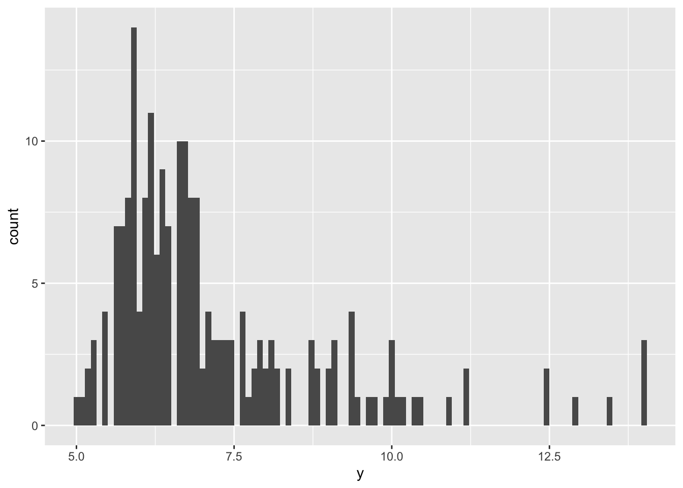
This is an instance where bootstrapping is handy. Bootstrapping takes a random sample of size n from your sample, and fits your model again. Then it resamples, and fits your model again…and again, and again. It samples with replacement, so you’ll have some observations that appear multiple times in each iteration, while other observations are missed. After it has resampled your data and fit your model many times, it aggregates the results and spits out a bootstrapped estimate, standard error, and confidence interval. Since each iteration was based off of slightly different observations, your result is less likely to be biased by skew, outliers, or other wonky distributions.
Below we can see the arguments taken by the boot::boot() function
str(boot)## function (data, statistic, R, sim = "ordinary", stype = c("i", "f", "w"),
## strata = rep(1, n), L = NULL, m = 0, weights = NULL, ran.gen = function(d,
## p) d, mle = NULL, simple = FALSE, ..., parallel = c("no", "multicore",
## "snow"), ncpus = getOption("boot.ncpus", 1L), cl = NULL)Most important are the first three:
data: the matrix or data frame you’re working withstatistic: a function that returns your statistic of interestR: the number of times you want to resample
For us, the statistics we’re interested in are the estimates returned from our linear model. But we want to format a new function so that it automatically returns just those coefficients, and not all the other info that comes with lm. We can create a small function to extract this info like so:
fun <- function(data, index){
 return(coef(lm(mod, data = data, subset = index)))
}
Here, mod is the model we fit above, data is (obviously) our data, and index is a vector indicating which observations (rows) from our data frame should be included. For example, if we select all of our rows, our output should be identical to the initial results:
fun(data, 1:200)## (Intercept) x1 x2 x3 x4
## 7.56804577 -0.37830562 -0.07984083 -0.06903943 0.84632682coef(mod)## (Intercept) x1 x2 x3 x4
## 7.56804577 -0.37830562 -0.07984083 -0.06903943 0.84632682boot() randomly chooses which observations should be included in index
boot.object <- boot(data, fun, 1000)
boot.object
##
## ORDINARY NONPARAMETRIC BOOTSTRAP
##
##
## Call:
## boot(data = data, statistic = fun, R = 1000)
##
##
## Bootstrap Statistics :
## original bias std. error
## t1* 7.56804577 0.0482331382 1.0726538
## t2* -0.37830562 -0.0117212441 0.2004917
## t3* -0.07984083 0.0024717868 0.2827149
## t4* -0.06903943 -0.0040158995 0.3152365
## t5* 0.84632682 -0.0005952484 0.2533492And boot.ci gives us our confidence intervals. Note that, if you are interested in multiple coefficients like we are, you have to specifically call that estimate using the index argument, where 1 calls t1* above (the intercept for us), 2 calls t2* (our estimate for x4) etc.
#this is the intercept
boot.ci(boot.object, conf = .95, type = c("norm", "basic", "bca"), index = 1)
## BOOTSTRAP CONFIDENCE INTERVAL CALCULATIONS
## Based on 1000 bootstrap replicates
##
## CALL :
## boot.ci(boot.out = boot.object, conf = 0.95, type = c("norm",
## "basic", "bca"), index = 1)
##
## Intervals :
## Level Normal Basic BCa
## 95% ( 5.417, 9.622 ) ( 5.506, 9.635 ) ( 5.500, 9.630 )
## Calculations and Intervals on Original Scale#this is for x1
boot.ci(boot.object, conf = .95, type = c("norm", "basic", "bca"), index = 2)## BOOTSTRAP CONFIDENCE INTERVAL CALCULATIONS
## Based on 1000 bootstrap replicates
##
## CALL :
## boot.ci(boot.out = boot.object, conf = 0.95, type = c("norm",
## "basic", "bca"), index = 2)
##
## Intervals :
## Level Normal Basic BCa
## 95% (-0.7595, 0.0264 ) (-0.7374, 0.0163 ) (-0.7717, -0.0188 )
## Calculations and Intervals on Original Scale#this is for x2
boot.ci(boot.object, conf = .95, type = c("norm", "basic", "bca"), index = 3)## BOOTSTRAP CONFIDENCE INTERVAL CALCULATIONS
## Based on 1000 bootstrap replicates
##
## CALL :
## boot.ci(boot.out = boot.object, conf = 0.95, type = c("norm",
## "basic", "bca"), index = 3)
##
## Intervals :
## Level Normal Basic BCa
## 95% (-0.6364, 0.4718 ) (-0.6590, 0.4673 ) (-0.6288, 0.4856 )
## Calculations and Intervals on Original ScaleTo return all of our coefficients and their associated CIs in a nice clean table, we can use the following formula:
CItable = function(mod, data, boot.object){
  pred = c(names(mod$coefficients))
  index = seq(1:length(pred))
  CIt = data.frame(index, pred)
  for (i in index){
    CI = boot.ci(boot.object, conf = 0.95, type = "norm", index = i)
    CIt$Estimate[i] = boot.object[["t0"]][[i]]
    CIt$SEboot[i] = apply(boot.object$t,2,sd)[i]
    CIt$lower.bound[i] = CI$norm[,2]
    CIt$upper.bound[i] = CI$norm[,3]}
  return(CIt)
}
Let’s walk through what this does.
As arguments, this function takes in our model of interest, our data, and boot.object, the object created above using the boot() function.
First, the function creates a vector called pred which consists of the names of the model coefficients.
pred = c(names(mod$coefficients))
pred
## [1] "(Intercept)" "x1" "x2" "x3" "x4"Next it creates an index object, which is just a sequence of the same length as pred.
index = seq(1:length(pred))
index
## [1] 1 2 3 4 5We put them together in a data frame.
CIt = data.frame(index, pred)
CIt
## index pred
## 1 1 (Intercept)
## 2 2 x1
## 3 3 x2
## 4 4 x3
## 5 5 x4Next, we initiate a for loop which goes through each value in index, and plugs that into the boot.ci() function. Below, we input our boot.object object from above and set i to 1 as an example.
CI = boot.ci(boot.object, conf = 0.95, type = "norm", index = 1)
CI
## BOOTSTRAP CONFIDENCE INTERVAL CALCULATIONS
## Based on 1000 bootstrap replicates
##
## CALL :
## boot.ci(boot.out = boot.object, conf = 0.95, type = "norm", index = 1)
##
## Intervals :
## Level Normal
## 95% ( 5.417, 9.622 )
## Calculations and Intervals on Original ScaleOk, here we have our output in terrible text format.
Next, we pull the estimate out of our boot object.
boot.object[["t0"]][[1]]## [1] 7.568046Note that the CIt$Estimate[i]= just adds this extracted value to the ith row of CIt in a new column called Estimate.
To get the standard errors, we need to take the standard deviation of the 1000 replications of each of our coefficients. Here, boot.object$t gives us a matrix with 5 columns (one for each coefficient), and 1000 rows (one for each repetition).
head(boot.object$t)## [,1] [,2] [,3] [,4] [,5]
## [1,] 7.875881 -0.4552777 -0.62879867 0.5926316 0.7166760
## [2,] 6.570837 -0.1225229 0.06779021 -0.1819644 0.7719799
## [3,] 8.439980 -0.5099639 0.04043891 -0.3494414 0.7018210
## [4,] 6.619611 -0.2054833 -0.38904491 0.3489171 0.9155234
## [5,] 7.717201 -0.5518786 0.39719526 -0.3515270 0.8313202
## [6,] 7.269340 -0.3767260 -0.54977758 0.3026698 1.1379344str(boot.object$t)## num [1:1000, 1:5] 7.88 6.57 8.44 6.62 7.72 ...The apply() function is a fast way to apply a given function over different parts of a matrix. It takes in the matrix boot.object, as well as a margin value (1 for rows, 2 for columns) indicating which parts of the matrix the function will be applied over. Finally, it takes the function, sd. The [i] subscripts specifies which column we are interested in according to our progression through the for loop. As an example:
apply(boot.object$t, 2, sd)[1]## [1] 1.072654Which matches the SE for the intercept from the overall boot object.
boot.object##
## ORDINARY NONPARAMETRIC BOOTSTRAP
##
##
## Call:
## boot(data = data, statistic = fun, R = 1000)
##
##
## Bootstrap Statistics :
## original bias std. error
## t1* 7.56804577 0.0482331382 1.0726538
## t2* -0.37830562 -0.0117212441 0.2004917
## t3* -0.07984083 0.0024717868 0.2827149
## t4* -0.06903943 -0.0040158995 0.3152365
## t5* 0.84632682 -0.0005952484 0.2533492Finally, we can pull the lower and upper bounds like so:
CI$norm[,2]## [1] 5.41745CI$norm[,3]## [1] 9.622176Note that you can opt for different types of bootstrapped CIs, like BCA or percentile. But the subscripts in the final few lines of the function may change because of the different outputs. You can double check which ones to use by running.
CI$norm## conf
## (Intercept) 0.95 5.41745 9.622176Here we can clearly see that the first column is our confidence level, the second column is the lower bound, and the third is the upper bound. If we’re interested in BCA CIs:
CI = boot.ci(boot.object, conf = 0.95, type = "bca", index = 1)
CI$bca
## conf
## [1,] 0.95 25.01 975.96 5.500238 9.629616We see there are some additional parameters in there, and we would want the 4th and 5th for our CI bounds.
Anyway, the estimate, SE, lower, and upper bounds are all added as columns to the original CIt object, and finally, we return our completed table with return(CIt)
Now when we run our shiny new function, we get a shiny new table which doesn’t give you carpal tunnel from copying and pasting it to wherever it’s going to live. We can also now easily see which parameters have CIs that exclude 0, and which don’t. While both x1 and x4 were significant in the original linear model, it looks like x1 was not a very robust finding, as it’s CI includes 0 here.
CItable(mod = mod, data = data, boot.object = boot.object)## index pred Estimate SEboot lower.bound upper.bound
## 1 1 (Intercept) 7.56804577 1.0726538 5.4174497 9.62217553
## 2 2 x1 -0.37830562 0.2004917 -0.7595409 0.02637217
## 3 3 x2 -0.07984083 0.2827149 -0.6364237 0.47179847
## 4 4 x3 -0.06903943 0.3152365 -0.6828758 0.55282870
## 5 5 x4 0.84632682 0.2533492 0.3503667 1.34347743Getting comfortable with functions can really take your R skills to the next level. If you want to learn more about creating your own, I recommend Roger Peng’s R Programming for Data Science and Jenny Bryan’s Stat 545 sites.