Here, I show how to simulate multilevel data, specifically intensive longitudinal (daily diary) data. Multilevel data poses some challenges for simulation because it violates assumptions of independence and analyses typically include estimation of random effects (e.g., each person may have their own intercept and slope). This tutorial assumes background knowledge of multilevel modeling and within- and between-person effects.
Once you understand how to simulate multilevel data, you can see how to incorporate it into power simulations here.
Like all data simulations, you will need to have an idea as to the general parameters for the data you intend to simulate (means, standard deviations, etc.) as well as how they relate to each other (e.g., the model). But multilevel data requires more parameters to do this than, say, a simple regression model.
For the present example, I will base the simulation on an existing dataset of people with type 2 diabetes to inform these parameters. You can read more about the original dataset here. Depending on what you are using your simulated data for, you may need to pull these parameters from existing literature or pilot data (e.g., if you are conducting an a priori power analysis to inform data collection).
We will use these packages in this tutorial:
library(nlme)
library(MASS)
library(tidyverse)

set.seed(4321)
Intro to the Data
Ok let’s look at the data.
head(diabetes, n = 15)## # A tibble: 15 × 10
## id time collaboration PosAff PA_within PA_between NegAff NA_within
## <dbl> <dbl> <dbl> <dbl> <dbl> <dbl> <dbl> <dbl>
## 1 1 0 4 2.67 0.333 -1.32 1.33 -0.0556
## 2 1 1 2 3 0.667 -1.32 1.33 -0.0556
## 3 1 2 2 3.33 1 -1.32 1 -0.389
## 4 1 3 2 3 0.667 -1.32 1.33 -0.0556
## 5 1 4 2 3 0.667 -1.32 1.67 0.278
## 6 1 5 4 2.33 0 -1.32 3 1.61
## 7 1 6 1 2.67 0.333 -1.32 1 -0.389
## 8 1 7 NA NA NA -1.32 NA NA
## 9 1 8 3 1.33 -1 -1.32 1 -0.389
## 10 1 9 2 2.33 0 -1.32 1 -0.389
## 11 1 10 3 1.33 -1 -1.32 1.33 -0.0556
## 12 1 11 2 1.67 -0.667 -1.32 1.33 -0.0556
## 13 1 12 3 1.33 -1 -1.32 1.33 -0.0556
## 14 1 13 NA NA NA -1.32 NA NA
## 15 2 0 5 5 0 1.35 1 0
## # … with 2 more variables: NA_between <dbl>, age <dbl>We’ve got this data in long format: each participant has one row for each day they completed a daily diary.
We have the following variables:
id: the participant IDtime: the day of the diary assessment (0 through 13, with some exceptions due to missing data and/or participant error)PosAff: daily positive affect (PA)PA_between: participant’s mean PA across the 14 days, centered around the grand meanPA_within: how much someone deviated from their own average PA on a given dayNegAff: daily negative affect (NA)NA_between: participant’s mean PA across the 14 days, centered around the grand meanNA_within: how much someone deviated from their own average NA on a given dayshared_appraisal: daily shared appraisal rating, or how much the person perceived their diabetes to be shared with their romantic partner on a given daycollaboration: daily collaboration rating, or the extent to which the participant collaborated with their romantic partner to manage their diabetes on that day.age: the participant’s age
Notice that we have three different variables for both positive and negative affect: the raw daily variable (PosAff and NegAff), the between-person variables, and the within-person variables. You can find some quick code for parsing the raw variable into within- and between-person effects here. Most important, notice that the between-person variables are the same across time for an individual, while the within-person variables change from day to day.
How many participants do we have?
diabetes %>%
  group_by(id) %>%
  summarise() %>%
  nrow()
## [1] 200Let’s say we are interested in whether mood predicts collaboration on a given day. We think that positive affect (PA) will predict collaboration. We also know that PA and negative affect (e.g., depressed mood or NA) overlaps with PA. So we want to control for NA when we are testing this hypothesis. We also want to control for participant age, because both PA and collaboration tend to increase as participants get older. We allow participants to randomly vary in their intercepts, as well as their slopes for time and PA_within.
Thus, the model we estimate using the original data is as follows:
collabMod <- lme(collaboration ~ PA_within + PA_between +
                   NA_within + NA_between + age + time,
                  data = diabetes,
                  random = ~ PA_within + time + 1|id,
                  na.action = na.omit)
Our task is to simulate a dataset that captures the same relationships identified in this model. The first crucial step is to write out your equation. Really, do this now – it will save a lot of headache later.
Here is the math behind the above model, broken down into level 1 (within-person) and level 2 (between-person) equations, where i represents an individual and j indicates a single assessment timepoint:
Level 1: \[collaboration_{ij} = \beta_{0j} + \beta_{1j}(PAwithin) + \beta_{2j}(NAwithin) + \beta_{3j}(time) + r_{ij} \]
Level 2: \[\beta_{0j} = \gamma_{00} + (\gamma_{01})PAbetween + (\gamma_{02}NAbetween) + (\gamma_{03})age + u_{0j} \] \[\beta_{1j} = \gamma_{10} + u_{1j} \] \[\beta_{2j} = \gamma_{20}\] \[\beta_{3j} = \gamma_{30} + u_{3j} \]
Combined and rearranged:
\[collaboration_{ij} = (\gamma_{00} + u_{0j}) + (\gamma_{10} + u_{1j})PAwithin + \] \[(\gamma_{20})NAwithin + (\gamma_{30} + u_{3j})time + (\gamma_{01})PAbetween +\] \[(\gamma_{02}NAbetween) + (\gamma_{03})age + r_{ij}\]
Looking at the combined model, \(\gamma\) (gamma) represents a fixed effect, and \(u\) represents a random effect. So, as we specified in our code above, we have random effects for the intercept (\(u_{0j}\)), as well as for the slopes of PA_within (\(u_{1j}\)) and time (\(u_{3j}\)). We’ll need all of these parameters to simulate our dependent variable, collaboration.
Ok, now let’s look at the full model output:
summary(collabMod)## Linear mixed-effects model fit by REML
## Data: diabetes
## AIC BIC logLik
## 6658.053 6739.37 -3315.027
##
## Random effects:
## Formula: ~PA_within + time + 1 | id
## Structure: General positive-definite, Log-Cholesky parametrization
## StdDev Corr
## (Intercept) 0.92056299 (Intr) PA_wth
## PA_within 0.34580651 0.141
## time 0.04764546 -0.300 0.394
## Residual 0.78970783
##
## Fixed effects: collaboration ~ PA_within + PA_between + NA_within + NA_between + age + time
## Value Std.Error DF t-value p-value
## (Intercept) 1.8529140 0.3176015 2265 5.834085 0.0000
## PA_within 0.0924109 0.0412089 2265 2.242501 0.0250
## PA_between 0.4127638 0.0954993 196 4.322164 0.0000
## NA_within -0.0026098 0.0354924 2265 -0.073532 0.9414
## NA_between -0.1358025 0.1361690 196 -0.997308 0.3198
## age 0.0112956 0.0058007 196 1.947279 0.0529
## time -0.0211969 0.0055048 2265 -3.850616 0.0001
## Correlation:
## (Intr) PA_wth PA_btw NA_wth NA_btw age
## PA_within 0.029
## PA_between 0.155 -0.021
## NA_within -0.005 0.372 -0.007
## NA_between -0.064 -0.001 0.545 -0.032
## age -0.974 -0.013 -0.164 0.002 0.062
## time -0.101 0.148 0.014 0.032 0.006 -0.002
##
## Standardized Within-Group Residuals:
## Min Q1 Med Q3 Max
## -3.59580931 -0.57825261 -0.08428441 0.54513978 4.19543636
##
## Number of Observations: 2468
## Number of Groups: 200There’s a lot of information here.
First, notice the random effects. We are given a standard deviation for each of our random effects, as well as for the residual. We also have a correlation matrix showing how these are related to each other.
Next, we see our fixed effects, including the estimate, SE, DF, t-value, and p-value. Below that, we see another correlation matrix representing how these fixed effects relate to each other.
So how do we start simulating a dataset that captures all of these relations represented in this model?
Starting Small
Let’s start small. We know that we want 200 participants, each with 14 days of diary data:
n_participants <- 200
n_timepoints <- 14
time <- rep(seq(0, n_timepoints-1, length = n_timepoints), n_participants)
id <- rep(1:n_participants, each = n_timepoints)

#put together into a data frame
sim_data <- data.frame(id, time)
head(sim_data, n = 20)
## id time
## 1 1 0
## 2 1 1
## 3 1 2
## 4 1 3
## 5 1 4
## 6 1 5
## 7 1 6
## 8 1 7
## 9 1 8
## 10 1 9
## 11 1 10
## 12 1 11
## 13 1 12
## 14 1 13
## 15 2 0
## 16 2 1
## 17 2 2
## 18 2 3
## 19 2 4
## 20 2 5Now let’s add our participants’ ages. What do participant ages look like in our observed sample?
diabetes %>%
  summarise(mean_age = mean(age, na.rm = T),
            sd_age = sd(age, na.rm = T))
## # A tibble: 1 × 2
## mean_age sd_age
## <dbl> <dbl>
## 1 53.4 11.2ggplot(diabetes, aes(x = age)) +
geom_histogram()## `stat_bin()` using `bins = 30`. Pick better value with `binwidth`.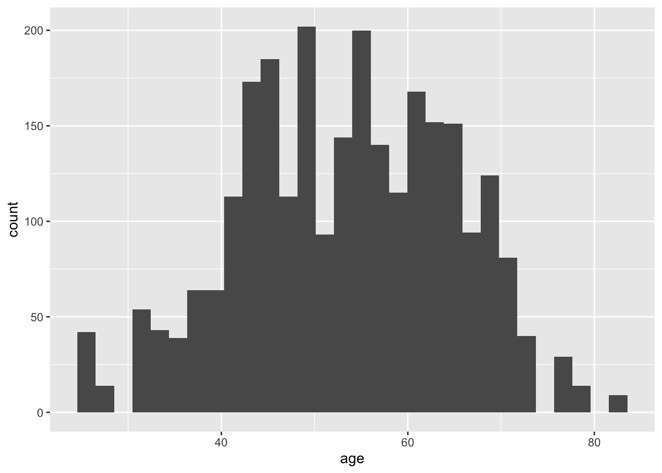
We can randomly sample from a normal distribution based on this mean, SD, and distribution shape.
sim_data$age <- rnorm(n_participants, mean = 53.40, sd = 11.25) %>%
  #let's just keep one decimal place
  round(1) %>%
  #repeat each age 14 times (age stays the same within a participant)
  rep(each = n_timepoints)

head(sim_data)
## id time age
## 1 1 0 48.6
## 2 1 1 48.6
## 3 1 2 48.6
## 4 1 3 48.6
## 5 1 4 48.6
## 6 1 5 48.6Ok, now let’s estimate our raw daily PosAff and NegAff variables.
Just like above, we’ll need the means and standard deviations from our original dataset:
diabetes %>% summarise(meanPA = mean(PosAff, na.rm = TRUE),
                       sdPA = sd(diabetes$PosAff, na.rm = TRUE),
                       meanNA = mean(NegAff, na.rm = TRUE),
                       sdNA = sd(NegAff, na.rm = TRUE))
## # A tibble: 1 × 4
## meanPA sdPA meanNA sdNA
## <dbl> <dbl> <dbl> <dbl>
## 1 3.66 1.04 1.49 0.810Again, we can randomly sample from a normal distribution based on these parameters. Note that this assumes PA and NA are statistically unrelated – which is almost certainly false. We’ll go with this for now, and below will look at how to simulate correlated independent variables.
sim_data$PosAff <-
  #each person gets a different score each day
  rnorm(n_participants*n_timepoints,
                     mean = 3.655, sd = 1.042)

sim_data$NegAff <- rnorm(n_participants*n_timepoints,
                       mean = 1.485, sd = .810)

head(sim_data)
## id time age PosAff NegAff
## 1 1 0 48.6 3.355986 2.1198075
## 2 1 1 48.6 2.982700 1.1057182
## 3 1 2 48.6 3.511898 2.0819549
## 4 1 3 48.6 2.143793 0.8968255
## 5 1 4 48.6 1.386186 1.1530269
## 6 1 5 48.6 5.605619 1.0946574Looks good! Now we just need to parse our raw mood variables into within- and between-person effects. If you are confused by this code, you can see how it works and why we parse the data like this here.
# parsing within- and between-person effects
sim_data <-  sim_data %>%
    group_by(id) %>%
    mutate(PA_14daymean = mean(PosAff, na.rm=TRUE),
           NA_14daymean = mean(NegAff, na.rm=TRUE))%>%
    mutate(PA_within = PosAff - PA_14daymean,
           NA_within = NegAff -NA_14daymean) %>%
    ungroup()%>%
    mutate(PA_grandm = mean(PA_14daymean, na.rm=TRUE),
           NA_grandm = mean(NA_14daymean, na.rm=TRUE)) %>%
    mutate(PA_between = PA_14daymean - PA_grandm,
           NA_between = NA_14daymean - NA_grandm) %>%
  select(-c(PA_14daymean, NA_14daymean, PA_grandm, NA_grandm))
#we can drop these variables--we only needed them to calculate the
#within and between-person effects

head(sim_data)
## # A tibble: 6 × 9
## id time age PosAff NegAff PA_within NA_within PA_between NA_between
## <int> <dbl> <dbl> <dbl> <dbl> <dbl> <dbl> <dbl> <dbl>
## 1 1 0 48.6 3.36 2.12 -0.226 0.520 -0.0854 0.112
## 2 1 1 48.6 2.98 1.11 -0.599 -0.494 -0.0854 0.112
## 3 1 2 48.6 3.51 2.08 -0.0703 0.482 -0.0854 0.112
## 4 1 3 48.6 2.14 0.897 -1.44 -0.703 -0.0854 0.112
## 5 1 4 48.6 1.39 1.15 -2.20 -0.447 -0.0854 0.112
## 6 1 5 48.6 5.61 1.09 2.02 -0.506 -0.0854 0.112Looks good!
dd_data Function
We can summarize everything we’ve done so far in the following function, which takes the number of participants and timepoints, and outputs a simulated data frame with id, time, age, PosAff, NegAff, PA_within, NA_within, PA_between, and NA_between.
dd_data <- function(n_participants, n_timepoints) {
  time <- rep(seq(1, n_timepoints, length = n_timepoints), n_participants)
  id <- rep(1:n_participants, each = n_timepoints)
  age <- runif(n_participants, min = 25, max = 82)
  sim_data <- data.frame(id, time, age = rep(age, each = n_timepoints))
  sim_data$PosAff <- rnorm(n_participants*n_timepoints, mean = 3.655, sd = 1.485)
  sim_data$NegAff <- rnorm(n_participants*n_timepoints, mean = 1.042, sd = .810)
  sim_data <-  sim_data %>% # parsing within- and between-person effects
    group_by(id) %>%
    mutate(PA_14daymean = mean(PosAff, na.rm=TRUE),
           NA_14daymean = mean(NegAff, na.rm=TRUE))%>%
    mutate(PA_within = PosAff - PA_14daymean,
           NA_within = NegAff -NA_14daymean) %>%
    ungroup()%>%
    mutate(PA_grandm = mean(PA_14daymean, na.rm=TRUE),
           NA_grandm = mean(NA_14daymean, na.rm=TRUE)) %>%
    mutate(PA_between = PA_14daymean - PA_grandm,
           NA_between = NA_14daymean - NA_grandm) %>%
    select(-c(PA_14daymean, NA_14daymean, PA_grandm, NA_grandm))
  return(sim_data)
}
Always good to test it:
dd_test <- dd_data(200, 14)
head(dd_test, n = 20)
## # A tibble: 20 × 9
## id time age PosAff NegAff PA_within NA_within PA_between NA_between
## <int> <dbl> <dbl> <dbl> <dbl> <dbl> <dbl> <dbl> <dbl>
## 1 1 1 38.0 4.62 1.35 1.27 0.157 -0.276 0.153
## 2 1 2 38.0 3.01 1.83 -0.344 0.639 -0.276 0.153
## 3 1 3 38.0 3.66 0.391 0.307 -0.800 -0.276 0.153
## 4 1 4 38.0 3.23 3.48 -0.119 2.29 -0.276 0.153
## 5 1 5 38.0 2.94 1.17 -0.409 -0.0242 -0.276 0.153
## 6 1 6 38.0 2.47 2.58 -0.883 1.39 -0.276 0.153
## 7 1 7 38.0 3.49 1.28 0.140 0.0881 -0.276 0.153
## 8 1 8 38.0 3.91 0.676 0.560 -0.515 -0.276 0.153
## 9 1 9 38.0 4.79 1.44 1.43 0.248 -0.276 0.153
## 10 1 10 38.0 3.56 -0.269 0.203 -1.46 -0.276 0.153
## 11 1 11 38.0 3.92 1.70 0.564 0.511 -0.276 0.153
## 12 1 12 38.0 2.05 1.05 -1.30 -0.140 -0.276 0.153
## 13 1 13 38.0 3.03 0.558 -0.324 -0.633 -0.276 0.153
## 14 1 14 38.0 2.26 -0.556 -1.09 -1.75 -0.276 0.153
## 15 2 1 45.3 3.61 1.35 -0.354 0.172 0.331 0.140
## 16 2 2 45.3 5.78 -0.0491 1.82 -1.23 0.331 0.140
## 17 2 3 45.3 3.97 1.89 0.0128 0.711 0.331 0.140
## 18 2 4 45.3 2.77 0.780 -1.19 -0.398 0.331 0.140
## 19 2 5 45.3 3.13 1.99 -0.831 0.814 0.331 0.140
## 20 2 6 45.3 3.80 2.18 -0.156 1.01 0.331 0.140Cool! Now we just need to estimate our dependent variable, collaboration, right? Unfortunately, no.
Adding Random Effects
This is where things get more complicated, because we need to add those random effects before estimating the outcomes variable. As a reminder, a random effect captures individual heterogeneity across our intercept and slope values. For example, while our output from our initial model tells us that our intercept is 1.85, our random intercept says that this value is actually variable across participants. How variable?
VarCorr(collabMod)## id = pdLogChol(PA_within + time + 1)
## Variance StdDev Corr
## (Intercept) 0.84743622 0.92056299 (Intr) PA_wth
## PA_within 0.11958214 0.34580651 0.141
## time 0.00227009 0.04764546 -0.300 0.394
## Residual 0.62363845 0.78970783This table shows us the variance and standard deviation of our random effects and residuals, as well as how they are related to each other (i.e., the correlations). For instance, we can see that the effect of time on our outcome really doesn’t change that much from person to person, but within-person PA does. We can also see that people with larger intercept random effects tend to have somewhat larger (r = .141) within-person PA random effects.
So what do we do with this information?
First, we need to pull the covariance matrix of the random effects, rather than the correlation matrix, because the covariance matrix takes into account the standard deviations (or variances) of each random effect.
For nlme models, the getVarCov function accomplishes this.
cov <- getVarCov(collabMod)
cov
## Random effects variance covariance matrix
## (Intercept) PA_within time
## (Intercept) 0.847440 0.044833 -0.0131510
## PA_within 0.044833 0.119580 0.0064890
## time -0.013151 0.006489 0.0022701
## Standard Deviations: 0.92056 0.34581 0.047645Then, we’ll use a function from the MASS packages called mvrnorm, which randomly samples from a multivariate normal distribution based on these covariances.
random_effects <- mvrnorm(n_participants, c(0,0,0), Sigma = cov)Note here that n = n_participants, rather than n_participants*n_timepoints. That is, random effects vary across people, not across within-person time points.
This results in a 3 by 200 random_effects matrix.
head(random_effects)## (Intercept) PA_within time
## [1,] 1.4632102 -0.31907004 -0.018897867
## [2,] 0.3884006 -0.07199089 -0.040755470
## [3,] -0.7905150 -0.33635644 -0.013735338
## [4,] -2.4296293 -0.28559102 0.067819419
## [5,] 0.4081169 -0.24265508 -0.007748071
## [6,] 0.1985533 0.54023222 0.007813314Each column is a random effect, each row represents a different person, and because of the way we sampled them, they should covary in the same way as the covariance matrix from the model:
cov(random_effects)## (Intercept) PA_within time
## (Intercept) 0.92708400 0.056000468 -0.013733531
## PA_within 0.05600047 0.131580572 0.005525947
## time -0.01373353 0.005525947 0.002251855Looks pretty close!
Recall our equations from above, especially our combined model:
\[collaboration_{ij} = (\gamma_{00} + u_{0j}) + (\gamma_{10} + u_{1j})PAwithin + \] \[(\gamma_{20})NAwithin + (\gamma_{30} + u_{3j})time + (\gamma_{01})PAbetween +\] \[(\gamma_{02}NAbetween) + (\gamma_{03})age + r_{ij}\]
We can see that the intercept and beta values for PA_within and time are simply the sum of a fixed effect, \(\gamma\), and a random effect, \(u\).
So all we need to do is to add our newly simulated random effects to the fixed effects from the original model.
You can pull these fixed effect coefficients from the model like so:
beta_int <-  fixed.effects(collabMod)["(Intercept)"]
beta_time <-  fixed.effects(collabMod)["time"]
beta_PA_within <- fixed.effects(collabMod)["PA_within"]
And combine them with the random effects like this:
#Pull out each column of random effects
rand_intercepts <- rep(random_effects[,1], each = n_timepoints)
rand_PA_within <- rep(random_effects[,2], each = n_timepoints)
rand_time <- rep(random_effects[,3], each = n_timepoints)


sim_data <- sim_data %>%
    mutate(intercepts = (beta_int + rand_intercepts),
           slope_time = (beta_time + rand_time),
           slope_PA_within = (beta_PA_within + rand_PA_within))
Notice that for each random effect, we have to repeat it n_timepoints times. This is because our sim_data data frame is in long format, where each person has a new line of data for each time point.
So now when we look at sim_data, we see the new variables intercepts, slope_time, and slope_PA_within each of which are different for different people:
sim_data %>%
  select(id, intercepts, slope_time, slope_PA_within) %>%
  head(n = 18)
## # A tibble: 18 × 4
## id intercepts slope_time slope_PA_within
## <int> <dbl> <dbl> <dbl>
## 1 1 3.32 -0.0401 -0.227
## 2 1 3.32 -0.0401 -0.227
## 3 1 3.32 -0.0401 -0.227
## 4 1 3.32 -0.0401 -0.227
## 5 1 3.32 -0.0401 -0.227
## 6 1 3.32 -0.0401 -0.227
## 7 1 3.32 -0.0401 -0.227
## 8 1 3.32 -0.0401 -0.227
## 9 1 3.32 -0.0401 -0.227
## 10 1 3.32 -0.0401 -0.227
## 11 1 3.32 -0.0401 -0.227
## 12 1 3.32 -0.0401 -0.227
## 13 1 3.32 -0.0401 -0.227
## 14 1 3.32 -0.0401 -0.227
## 15 2 2.24 -0.0620 0.0204
## 16 2 2.24 -0.0620 0.0204
## 17 2 2.24 -0.0620 0.0204
## 18 2 2.24 -0.0620 0.0204Now the last thing we need to take into account is our residual, or error term, \(r_{ij}\). Just as the subscript indicates, this does vary across time points. We can pull \(\sigma\), the SD of our residual directly from the model, and use it to randomly sample from a normal distribution with a mean of 0.
sigma <-  collabMod[["sigma"]]
error <- rnorm(n_participants*n_timepoints, 0, sigma)

#add to the data frame
sim_data <- sim_data %>%
  mutate(error)

sim_data %>% select(id, error) %>%
  head()
## # A tibble: 6 × 2
## id error
## <int> <dbl>
## 1 1 0.742
## 2 1 -0.364
## 3 1 -1.45
## 4 1 0.104
## 5 1 -0.650
## 6 1 0.289get_random_effects Function
We can summarize all of this syntax used to create the random effects in the following function, which takes as arguments the sim_data from our dd_dat function, the numbers of participants and time points, and the original nlme model:
get_random_effects <- function(sim_data, n_participants,
                                n_timepoints, nlme.model){
  beta_int <-  fixed.effects(nlme.model)["(Intercept)"]
  beta_time <-  fixed.effects(nlme.model)["time"]
  beta_PA_within <- fixed.effects(nlme.model)["PA_within"]
  sigma <-  nlme.model[["sigma"]]
  cov <- getVarCov(nlme.model)
  a <- mvrnorm(n_participants, c(0,0,0), Sigma = cov)
  rand_intercepts <- rep(a[,1], each = n_timepoints)
  rand_PA_within <- rep(a[,2], each = n_timepoints)
  rand_time <- rep(a[,3], each = n_timepoints)
  error <- rnorm(n_participants*n_timepoints, 0, sigma)
  sim_data <- sim_data %>%
    mutate(intercepts = (beta_int + rand_intercepts),
           slope_time = (beta_time + rand_time),
           slope_PA_within = (beta_PA_within + rand_PA_within),
           error)
  return(sim_data)
}
Are we done yet?
get_outcome Function
Not quite! Now we can (finally) calculate our independent variable, collaboration. To do so, we plug in our combined equation from above:
get_outcome <- function(sim_data, n_participants,
                             n_timepoints, nlme.model){
  #betas for predictors with only fixed effects:
  beta_PA_between <- fixed.effects(nlme.model)["PA_between"]
  beta_NA_within <- fixed.effects(nlme.model)["NA_within"]
  beta_NA_between <- fixed.effects(nlme.model)["NA_between"]
  beta_age <- fixed.effects(nlme.model)["age"]
  sim_data <- sim_data %>%
    #this should match combined model above:
    mutate(collaboration =
             intercepts +
             slope_PA_within*PA_within +
             beta_PA_between*PA_between +
             beta_NA_within*NA_within +
             beta_NA_between*NA_between +
             slope_time*time +
             beta_age*age +
             error)
  return(sim_data)
}
Note that we still need to pull the coefficients for predictors with fixed effects only. As fixed effects, these slopes are the same across all participants, so don’t need to be added into our data frame as new columns.
Putting it all together
Now we can combine our three functions dd_data, get_random_effects and get_outcome into one sleek simulate_data function:
simulate_data <- function(n_participants, n_timepoints, nlme.model){
  dd_data(n_participants, n_timepoints) %>%
    get_random_effects(n_participants, n_timepoints, nlme.model) %>%
    get_outcome(n_participants, n_timepoints, nlme.model)
}
Let’s recap everything that is going on here. We input the number of participants, number of time points, and original nlme model. dd_dat takes just n_participants and n_timepoints and outputs the sim_data data frame where each participant has 14 lines of data on our predictors of interest. get_random_effects takes this sim_data and adds random effects for intercepts, time, and PA_within, and outputs a modified sim_data object. Finally, get_outcome uses sim_data and some additional information from our model to estimate our outcome based on our combined model.
(Remember that the pipe, %>% , takes the output of a line and inputs it as the first argument in the next line. That’s why we don’t have to type sim_data as an input – it’s being passed through each function under the hood.)
Now we can run this function, and use the resulting data frame to fit our original model. This new output should closely match the original output.
sim_test <- simulate_data(200, 14, collabMod)simMod <- lme(collaboration ~ PA_within + PA_between +
NA_within + NA_between + age + time,
data = sim_test,
random = ~ PA_within + time + 1|id,
na.action = na.omit)summary_fixed <- function(nlme.mod){
summary(nlme.mod)[["tTable"]] %>%
as.data.frame() %>%
select(Value, Std.Error, "p-value") %>%
rename(p = "p-value") %>%
mutate(
Value = round(Value, 2),
Std.Error = round(Std.Error, 2),
p = round(p, 3))
}
summary_fixed(collabMod)## Value Std.Error p
## (Intercept) 1.85 0.32 0.000
## PA_within 0.09 0.04 0.025
## PA_between 0.41 0.10 0.000
## NA_within 0.00 0.04 0.941
## NA_between -0.14 0.14 0.320
## age 0.01 0.01 0.053
## time -0.02 0.01 0.000summary_fixed(simMod)## Value Std.Error p
## (Intercept) 1.91 0.23 0.000
## PA_within 0.04 0.03 0.130
## PA_between 0.32 0.17 0.064
## NA_within -0.01 0.02 0.697
## NA_between 0.45 0.31 0.148
## age 0.01 0.00 0.007
## time -0.03 0.01 0.000Looks pretty good! Notice that the non-significant predictors (like NA_between) are quite different across the two models, while the significant predictors match.
We can also compare the random effects:
VarCorr(collabMod)## id = pdLogChol(PA_within + time + 1)
## Variance StdDev Corr
## (Intercept) 0.84743622 0.92056299 (Intr) PA_wth
## PA_within 0.11958214 0.34580651 0.141
## time 0.00227009 0.04764546 -0.300 0.394
## Residual 0.62363845 0.78970783VarCorr(simMod)## id = pdLogChol(PA_within + time + 1)
## Variance StdDev Corr
## (Intercept) 0.912248071 0.95511678 (Intr) PA_wth
## PA_within 0.140996279 0.37549471 0.143
## time 0.002571546 0.05071042 -0.240 0.332
## Residual 0.583742629 0.76403052Looks good! Now, you can use the simulate_data function in other analyses, like in Monte Carlo power simulations where you need to simulate data over and over again. To learn more about this, see my tutorial here.
Simulating dependent predictors
If you read through all of this and said to yourself, “Hm, I really wish this was more complicated,” then never fear, we can add another layer of complexity.
Above, we talked about how our positive and negative affect predictors are probably related to each other. That is, if someone reports feeling very happy on one day, they are probably also reporting very little sadness on that day. The way we have simulated this so far does not take this covariance into account. To see how to do this, see this tutorial, which uses the same sample data and model used here.